Introductory RL

Reinforcement learning (RL) is a way of training an agent to make sequences of decisions by finding the optimal action-taking policy through trial and error interactions with the environment. It is a powerful tool for solving complex problems in robotics, finance, and gaming. To broaden my knowledge in ML, I worked on a few small projects to learn fundamental deep RL algorithms such as (Double) DQN, REINFORCE, DDPG, and PPO. Please see this project if you are interested in NEAT and Pong instead.

I won’t be including the math here but it is essential to learn the whole theory behind RL before diving into implementation. I will link sources for those interested.

What is RL?

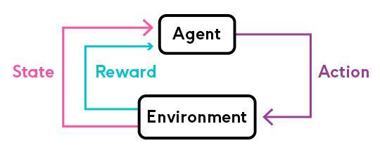
The agent learns to maximize the total reward by learning a policy that maps states to actions. The agent interacts with the environment by observing the state, taking an action, and receiving a reward. The agent then updates its policy based on the reward it receives.

The agent learns a deterministic (e.g. DDPG) or stochastic (e.g. REINFORCE, PPO) policy:

$$ \pi(s) = a \text{ or } \pi(a|s) = P(a|s) $$

A mathematical framework for RL is the Markov Decision Process (MDP), which consists of state space, action space, transition probabilities, reward function, and discount factor.

$$ < S, A, P, R, \gamma > $$

Deep Q Learning (DQN)

I coded a DQN agent that learns to trade stocks in my own custom environment built with OpenAI Gym API. The agent trains on historical data (yfinance API) and learns to maximize portfolio return by buying and selling stocks. We used a simple Sortino ratio as the reward function to penalize downside risk.

RL is especially suitable for time series data due to its sequential nature.

$$ \text{Sortino Ratio} = \frac{R_p - R_f}{\sigma_d} $$

The agent includes the following components:

• Experience Replay
• Epsilon Greedy Policy and Soft Update
• Target and Policy Networks

For the network, we chose a customized GRU network as follows (assuming you are familiar with PyTorch):

1def **init**(self, input_size, output_size):
2super(GDQN, self).**init**()
3self.gru1 = nn.GRU(input_size=input_size, hidden_size=HIDDEN_SIZE_GRU, num_layers=NUM_LAYERS_GRU, batch_first=True)
4self.dropout1 = nn.Dropout(p=DROPOUT)
5self.gru2 = nn.GRU(input_size=HIDDEN_SIZE_GRU, hidden_size=HIDDEN_SIZE_GRU, num_layers=1, batch_first=True)
6self.dropout2 = nn.Dropout(p=DROPOUT)
7self.fc = nn.Linear(HIDDEN_SIZE_GRU, output_size)

To train the agent, for each episode we let the agent interact with the environment for a fixed number of steps. The agent observes the state, takes an action, and receives a reward. We store the experience in a replay buffer and sample a batch to train the network.

Essentially, the agent is trying to minimize this loss function (Bellman equation) in order to learn a function that predicts the Q-value of each action given a state:

$$ \text{Loss} = \mathbb{E}[(Q(s, a) - (r + \gamma \max_{a’} Q(s’, a’))^2] $$

Subsequently the agent can choose the best action using the trained policy network:

$$ \pi(s) = \arg\max_a Q(s, a; \theta) $$

Here is how you can train the agent, for each episode:

 1# Initialize the environment and state
 2
 3state = self.env.reset()[0]
 4state = torch.tensor(state, dtype=torch.float32, device=self.device).unsqueeze(0)
 5for t in count():
 6action = self.select*action(state)
 7observation, reward, terminated, truncated, * = self.env.step(action.item())
 8reward = torch.tensor([reward], device=self.device, dtype=torch.float32)
 9done = terminated or truncated
10
11    if terminated:
12        next_state = None
13    else:
14        next_state = torch.tensor(observation, dtype=torch.float32, device=self.device).unsqueeze(0)
15
16    # Store the transition in memory
17    self.memory.push(state, action, next_state, reward)
18    state = next_state
19    self.optimize_model() # on the policy network
20
21    # soft update target network weights
22    target_net_state_dict = self.target_net.state_dict()
23    policy_net_state_dict = self.policy_net.state_dict()
24    for key in target_net_state_dict:
25        target_net_state_dict[key] = TAU * policy_net_state_dict[key] + (1 - TAU) * target_net_state_dict[key]
26    self.target_net.load_state_dict(target_net_state_dict)
27
28    if done:
29        # duration is how long it took to run that episode
30        episode_durations.append(t + 1)
31        plot_durations(episode_durations)
32        break

This project is based on this research paper

PPO and DDPG

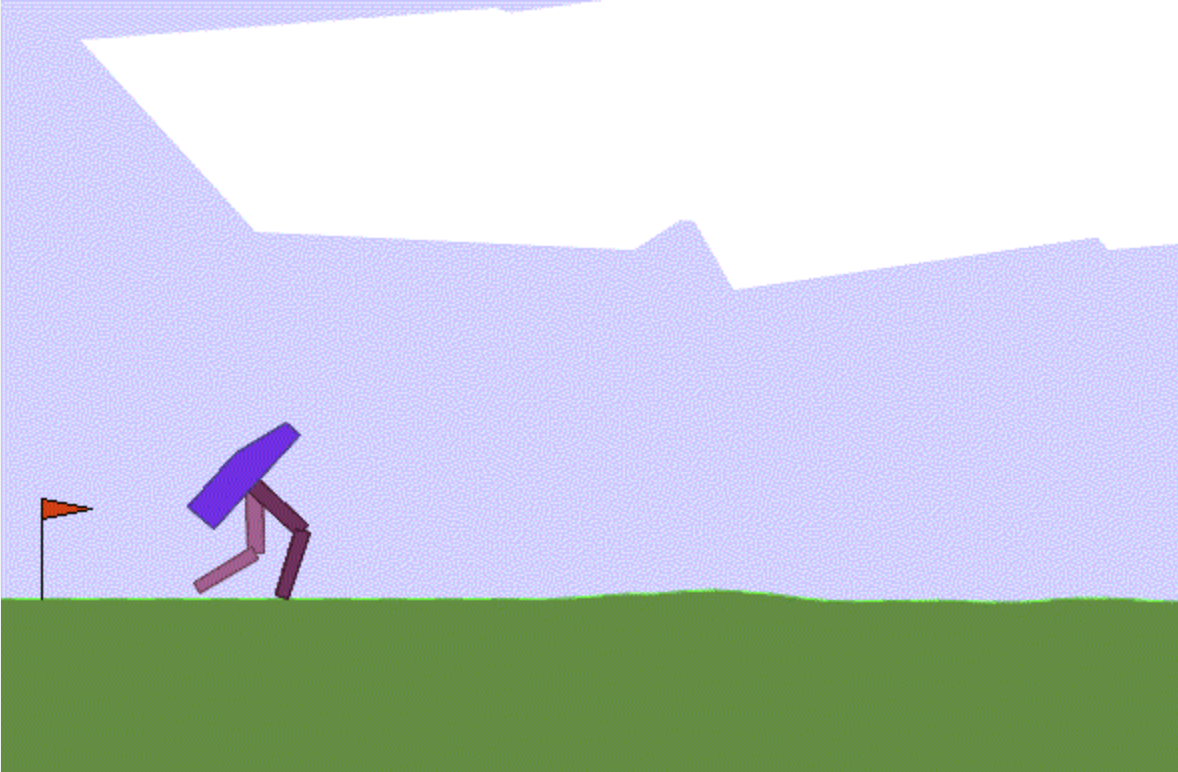
As part of my design team work, I continued my RL journey by implementing Proximal Policy Optimization (PPO) and Deep Deterministic Policy Gradients (DDPG) agents in simple control simulation games to learn how policy gradients work. These environments are all provided by the OpenAI Gym API:

• CartPole-v1
• Pendulum-v0
• MountainCar-v0
• LunarLander-v2
• BipedalWalker-v3

Compared to DQN, PG methods are more stable and efficient for continuous action spaces. However, they are more complicated and will take longer to learn. Policy gradient algorithms update the policy network in the direction that increases the probability of good actions and decreases the probability of bad actions, using the gradient of the expected return with respect to the policy parameters.

$$ \nabla_\theta J(\pi_\theta) = \mathbb{E} \left[ \sum_{t=0}^T \nabla_\theta \log \pi_\theta(a_t \mid s_t) \cdot R_t \right] $$

This can then be used to update the policy network using gradient ascent:

$$ \theta \leftarrow \theta + \alpha \nabla_{\theta} J(\theta) $$

The PPO agent in my implementation (based on OpenAI’s research paper) uses a “clipped surrogate objective” to prevent the agent from updating too much in one direction (which looks really scary at first):

$$ L^{\text{CLIP}}(\theta) = \mathbb{E}_t \left[ \min \left( r_t(\theta) A_t, \text{clip}(r_t(\theta), 1 - \epsilon, 1 + \epsilon) A_t \right) \right] $$

$$ \text{where } r_t(\theta) = \frac{\pi_\theta(a_t | s_t)}{\pi_{\theta_{\text{old}}}(a_t | s_t)} $$

Essentially, the agent is trying to maximize the expected return by updating the policy network in the direction that increases the probability of good actions and decreases the probability of bad actions. However, the clipping prevents the policy from making overly large updates, which could destabilize training or cause the agent to forget previously learned behaviors. This ensures more stable and reliable learning by constraining the change in the policy’s probability ratio within a safe range of

$$[1 - \epsilon, 1 + \epsilon]$$

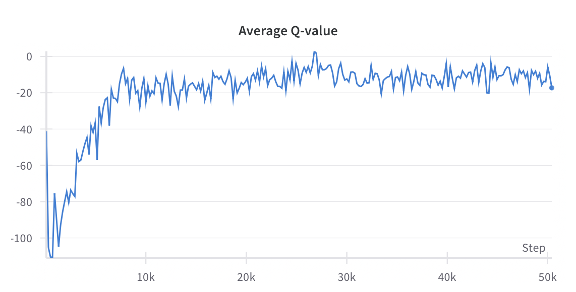
I included the two analytic plots (tracked using wandb) from training PPO on Cartpole, one of the simplest classic control games (balancing a pole on a cart):

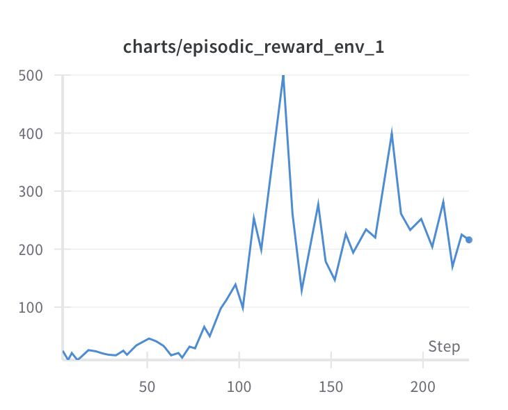
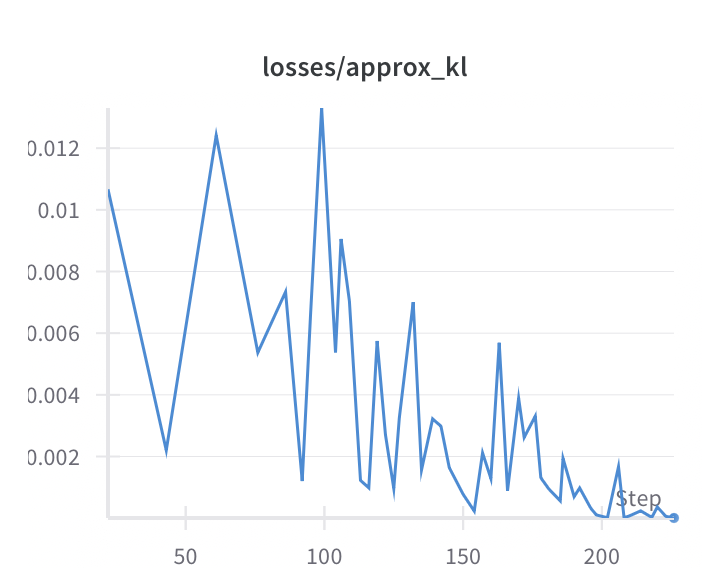
An increasing reward and decreasing KL divergence indicate that the agent is learning to balance the pole effectively. To be particular, the KL divergence measures the difference between the old and new policy, and a small value indicates that the policy is not changing too much, which is the advantage of PPO.

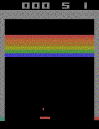
A note on Atari preprocessing

I find it helpful to note that these preprocessing techniques are useful when adapting RL algorithms to Atari games such as BreakoutNoFrameskip-v4:

 1# note: this assumes you use vectorized gym environments (since it's for ppo)
 2
 3def make_env(gym_id, seed, idx, capture_video, run_name):
 4    def thunk():
 5        env = gym.make(gym_id)
 6        env = gym.wrappers.RecordEpisodeStatistics(env)
 7        if capture_video:
 8            if idx == 0:
 9                env = gym.wrappers.RecordVideo(env, f"videos/{run_name}")
10                env = NoopResetEnv(env, noop_max=30) # no-op for a random number of steps, adds stochasticity
11                env = MaxAndSkipEnv(env, skip=4) # skip 4 frames and repeat the action to save computation
12                env = EpisodicLifeEnv(env) # end the episode when a life is lost
13        if "FIRE" in env.unwrapped.get_action_meanings():
14            env = FireResetEnv(env) # press FIRE button at the beginning of the episode
15            env = ClipRewardEnv(env) # clip the reward to -1, 0, 1 # original: 210x160x3, resized: 84x84x4
16            env = gym.wrappers.ResizeObservation(env, (84, 84)) # resize the observation to 84x84
17            env = gym.wrappers.GrayscaleObservation(env) # convert the observation to grayscale
18            env = gym.wrappers.FrameStackObservation(env, 4) # stack 4 frames together
19            env.action_space.seed(seed)
20            env.observation_space.seed(seed)
21        return env
22    return thunk

Resources

• Reinforcement Learning: An Introduction by Richard S. Sutton and Andrew G. Barto (Textbook)

• OpenAI Spinning Up (Tutorials with code)

• DeepMind X UCL (Lectures)

• RL notes (Notes)

• The following research papers to understand popular RL algorithms:

  • Playing Atari with Deep Reinforcement Learning

  • Human-level control through deep reinforcement learning

  • Continuous control with deep reinforcement learning

  • Proximal Policy Optimization Algorithms

  • High-Dimensional Continuous Control Using Generalized Advantage Estimation